
Latest News

AI Generated Newscast About Alien-Looking Sea Babies—What Are These Xenomorph Larvae Hiding?
HOOK: An alien-like sea creature has kept its adult form hidden for over a century, baffling scientists!The latest research reveals that mysterious baby facetot ...
AI Generated Newscast About Tesla’s FSD Shocker—$12k Gamble Leaves Owners Stunned!
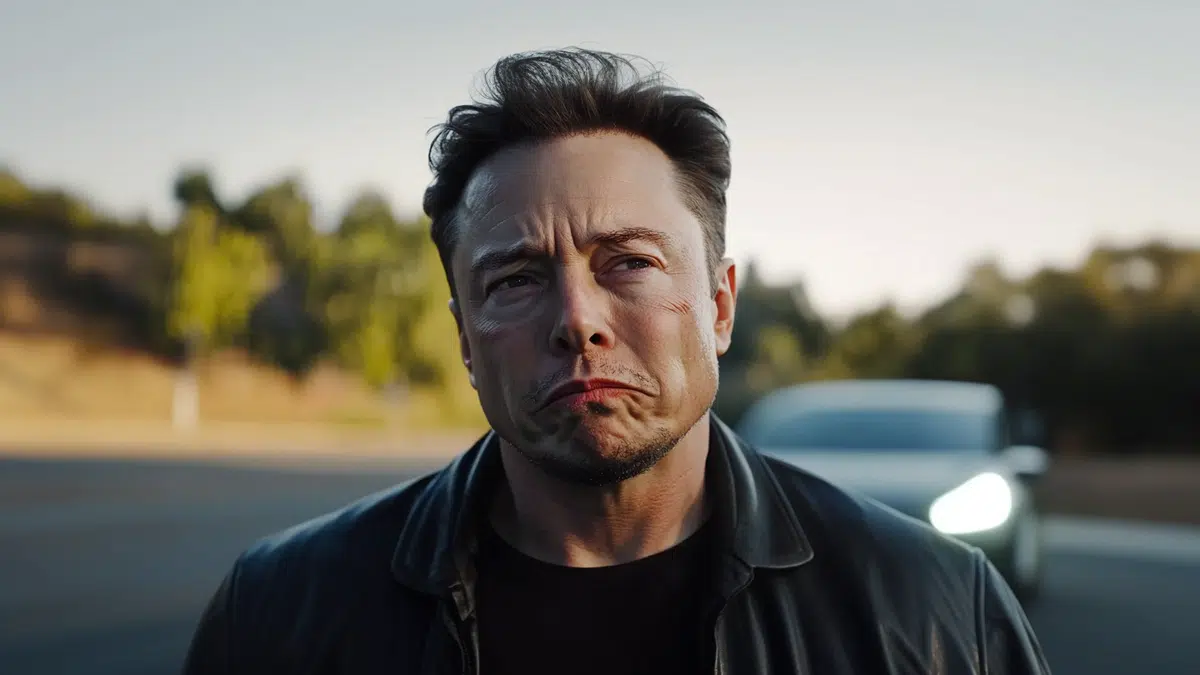
Would you spend $12,000 for a self-driving future, only to realize you’re not even close? That’s the shock Tesla owners are facing today.Elon Musk has admit ...
AI Generated Newscast About Asteroid 2025 FA22: NASA Warns of Close Encounter!
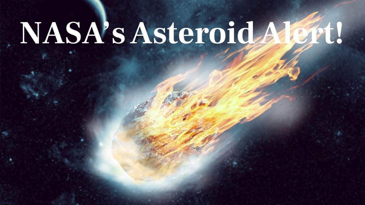
Brace yourselves: a giant asteroid is hurtling past Earth soon—are we truly safe? The AI generated newscast about asteroid 2025 FA22 reveals that this 520-foo ...

AI Generated Newscast About Solo Female Travel in India: Shocking Truth Revealed!
Would you dare to visit a place everyone warns you about? Em did—and what she discovered in Mumbai is eye-opening.This AI generated newscast about solo female ...
AI Generated Newscast About Strip Club Tax Bribery: Executives Busted in $8M Scandal!
Imagine dodging $8 million in taxes with free trips and private dances – only to have an AI generated newscast about your strip club scandal go viral.RCI Hosp ...
AI Generated Newscast About Virgin Australia Breastfeeding Scandal Leaves Viewers Stunned
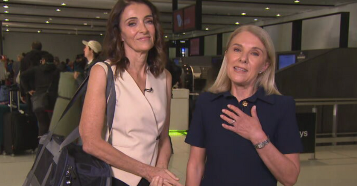
Imagine being shamed for feeding your babies in 2024 – that’s what lit up the internet after this AI generated newscast about Virgin Australia broke the sto ...

AI generated newscast about Star Going Supernova! V Sagittae’s Imminent Explosion Will Dazzle Earth
Could a cosmic explosion light up our sky brighter than the moon? The answer is yes, and it might happen soon! Scientists have cracked the secret of V Sagittae, ...
AI Generated Newscast About CPR in Space: Astronauts Face Shocking Medical Danger!
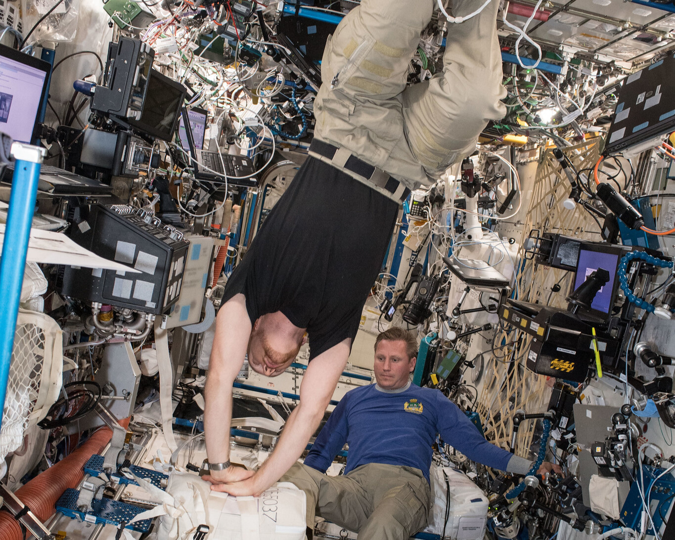
Imagine your heart stops… on the Moon. Would anyone know how to save you?This AI generated newscast about CPR in space reveals that traditional, manual CPR is ...
AI Generated Newscast About Tesla Trapped Kids: Parents Forced to Smash Windows?!
Would you be ready to smash your own car window to save your child? Some parents had to, after being trapped by Tesla’s high-tech doors—a story now under fe ...

AI Generated Newscast About Mysterious Planet Y: Did We Just Find the Next Big Planet in Our Solar System?
What if our solar system is hiding a secret planet right now? A new AI generated newscast about the Kuiper Belt reveals that scientists have found tantalizing e ...

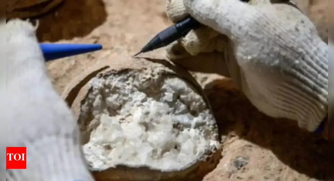
AI Generated Newscast About Ancient Comet: Did a Cosmic Catastrophe Erase Early America?
Did an ancient cosmic explosion wipe out America's first great culture in an instant? The AI generated newscast about this shocking discovery reveals that 'sho ...

AI Generated Newscast About NASA’s Shocking Spy Agency Transformation: Is Science Dead?
What if the agency that put humans on the Moon became a covert spy agency? That’s now reality.The Trump administration has reclassified NASA, shifting its mai ...
AI Generated Newscast About Burner Phones: Shocking Truth Behind Your Privacy Risks!
What if your phone could be used to track your every move—without you even knowing? This AI generated newscast about burner phones reveals how authorities wor ...

AI Generated Newscast About Mark Zuckerberg's MMA Obsession Shocking Meta Employees!
Would you wrestle your boss if it meant keeping your job? The latest AI generated newscast about Meta reveals Mark Zuckerberg has literally brought his MMA obse ...

AI Generated Moon Newscast: The Shocking Truth About Earth’s Fading Celestial Partner!
What if I told you the moon is sliding away from Earth—forever changing our days? The AI generated newscast about the moon reveals our lunar companion drifts ...

AI Generated Newscast About Deepest Black Egg Capsules Found – Flatworms Break Ocean Records!
Imagine a world so extreme, only the toughest creatures survive—now scientists have found black egg capsules deeper than ever before! In a mind-blowing discov ...
AI Generated Newscast About Dinosaur Eggs: Scientists Stunned by Atomic Dating Breakthrough!
Imagine unlocking the birth date of a dinosaur egg to the exact millionth year—it just happened. In a groundbreaking study, Chinese scientists used atomic-lev ...

AI Generated Newscast About Arctic Diatoms: Tiny Skaters That Could Save The Planet?!
Did you know the Arctic is full of microscopic skaters gliding through ice, defying what we thought possible? In this AI generated newscast about Arctic diatoms ...

AI Generated Newscast About Chrome vs. Edge: Microsoft’s Shocking Browser War Escalates!
Is your browser keeping you safe, or just selling you a story? Microsoft is once again pushing hard for users to pick Edge over Chrome, using bold new ads and i ...
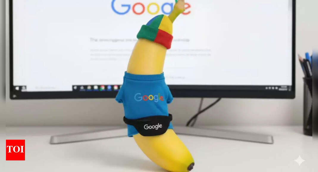
AI Generated Newscast About Nano Banana: The Viral 3D Photo Craze Everyone’s Addicted To!
What if you could see yourself, your pets, or your childhood memories as lifelike 3D figurines—instantly? The latest viral sensation, AI generated newscast ab ...
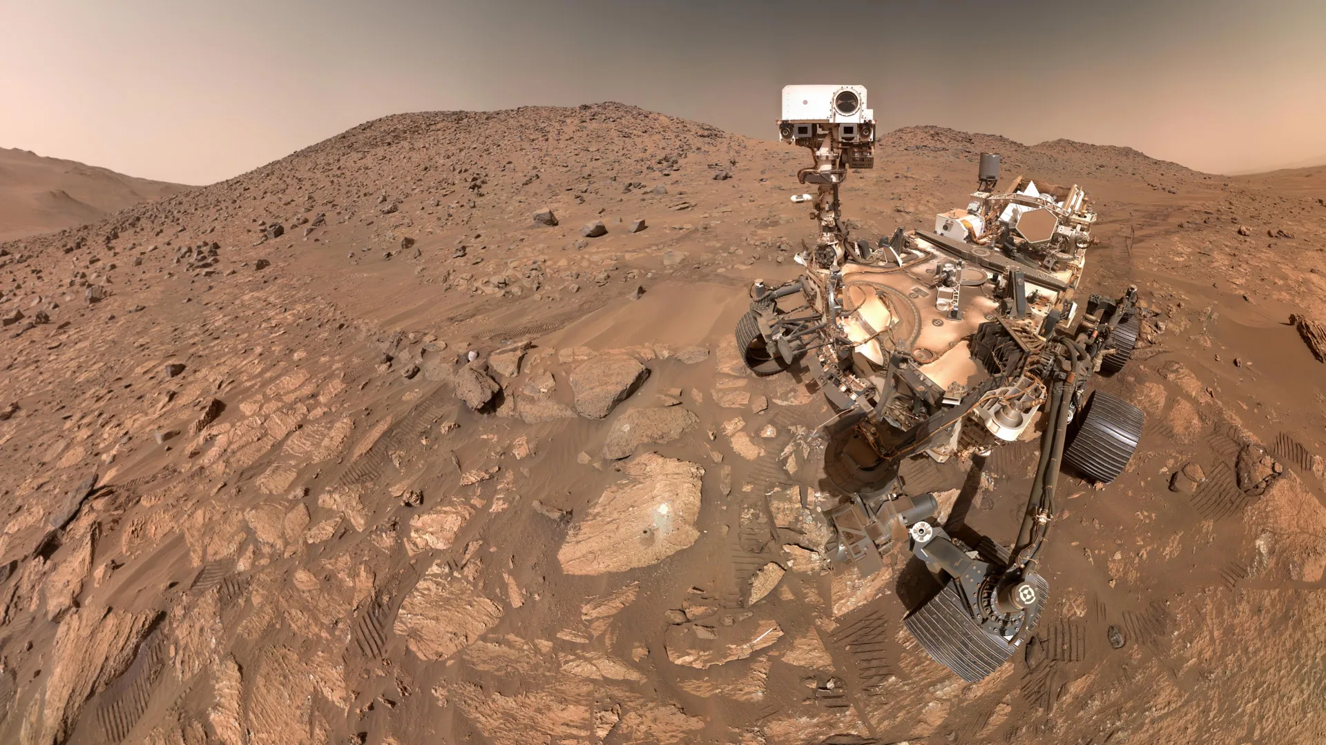
AI Generated Newscast About Mars: Shocking Signs of Ancient Life Discovered?
What if the first real evidence of Martian life was hiding in a single rock? That’s exactly what NASA’s Perseverance rover may have uncovered. A sample from ...

AI Generated Newscast About Central Park Bangkok Escalators: Why Everyone Is Obsessed!
Could an escalator really go viral and become the city’s most sought-after photo spot? Central Park Bangkok’s dazzling escalators have done just that, drawi ...
AI Generated Job Loss SHOCK: Google’s Hidden Layoffs Expose a Troubling AI Future!
Imagine training an AI, only to be laid off as it takes your job—that’s what just happened to over 200 Google contractors. In an AI generated newscast about ...
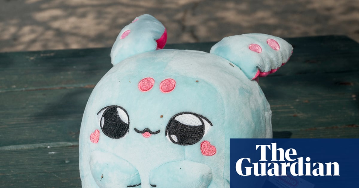
AI Generated Toy Shocks Parents: Is Your Child’s Best Friend Spying on Them?
Would you trust an AI plushie to raise your child? Grem, the AI-powered alien toy, just proved how complicated that question really is.The AI generated newscast ...
AI Generated Saree Edits: Creepy Secrets, Viral Fun & Hidden Dangers Revealed!
Can AI-generated saree edits reveal secrets you never meant to share? The AI generated newscast about Google Gemini’s Nano Banana AI has gone viral, but users ...

AI Generated Newscast About Soup Shocker: Teens Fined $300K for Hotpot Prank!
What happens when a drunken prank goes viral? You pay a $300,000 price tag and shock a nation. Two Chinese teens who urinated in a hotpot at Haidilao—and post ...
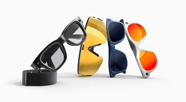
AI Generated Newscast About Meta's Secret Smart Glasses Leak – Shocking HUD Features Revealed!
Did Meta just leak its own future? An AI generated newscast about Meta’s smart glasses showcases a stunning new line of eyewear, including the mysterious Hype ...
AI Generated Newscast About CEO Scandal: Super Retail’s Shocking Leadership Shake-Up!
An explosive update rocks Super Retail Group as CEO Anthony Heraghty is fired on the spot after revelations about an office romance. A sudden board decision, tr ...

AI Generated Newscast About Search Wars: Is Google Losing to ChatGPT? Shocking Stats Reveal All!
AI-powered chatbots like ChatGPT are rapidly changing how we search online, threatening Google’s long-standing dominance. Across the world, users are turning ...
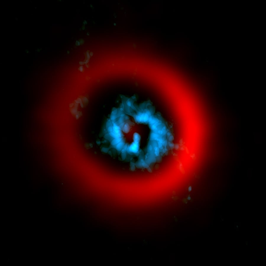
AI Generated Newscast About Protoplanets: Scientists Catch a Planet Being Born—LIVE!
You won’t believe it, but astronomers just caught a giant planet being born, right before our eyes! Using advanced telescopes, researchers observed AB Aurigae ...
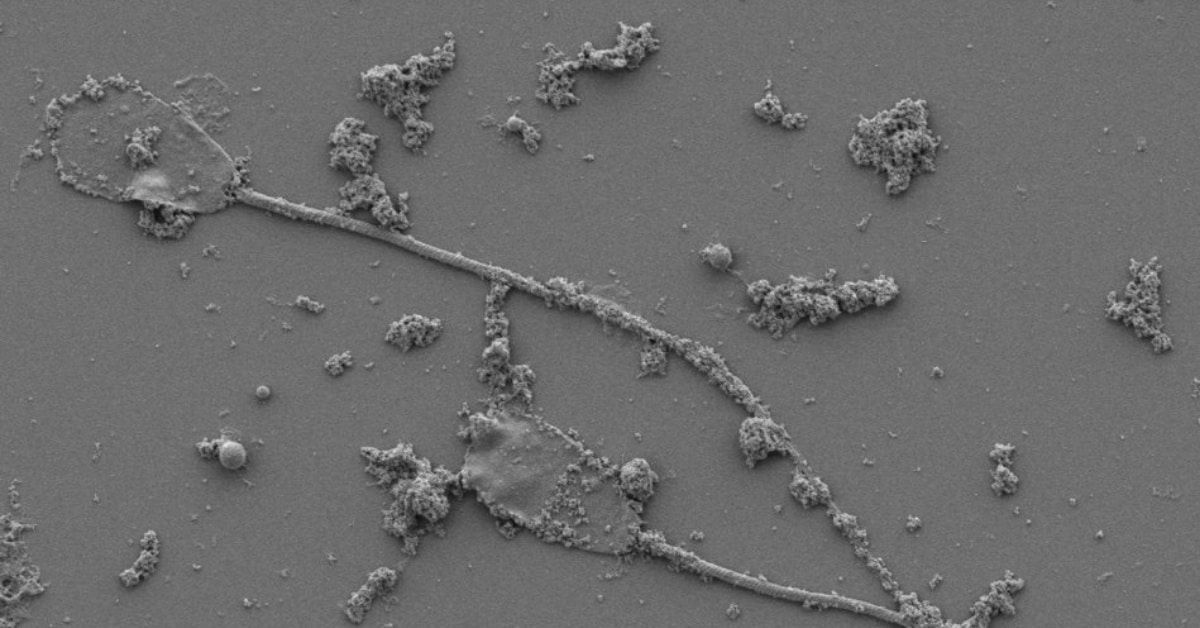
AI Generated Spermbots: Scientists Shock the World with Remote-Controlled Sperm!
Sperm cells as tiny, remote-controlled robots? It sounds like science fiction, but it’s real! In this AI generated newscast about sperm microrobots, researche ...
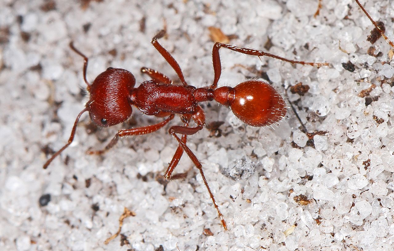
AI Generated Newscast About Ant Queen’s Shocking Double Species Offspring Revealed!
An ant queen just did the unthinkable—she gave birth to two different species at once, and scientists are stunned. In southern Europe, researchers studying Ib ...

AI Generated Newscast About Hacked Vape Pens: You Won’t Believe What’s Inside!
What if your next website was powered by a discarded vape pen? In an amazing example of tech ingenuity, hacker Bogdan Ionescu repurposed a throwaway vape's tiny ...

AI Generated Cyborg Cockroach Swarm: The Shocking Future of Disaster Rescue Revealed!
Would you ever trust a cockroach to save your life? Singapore’s NTU has unveiled the world’s first AI generated newscast about cyborg cockroaches, where the ...
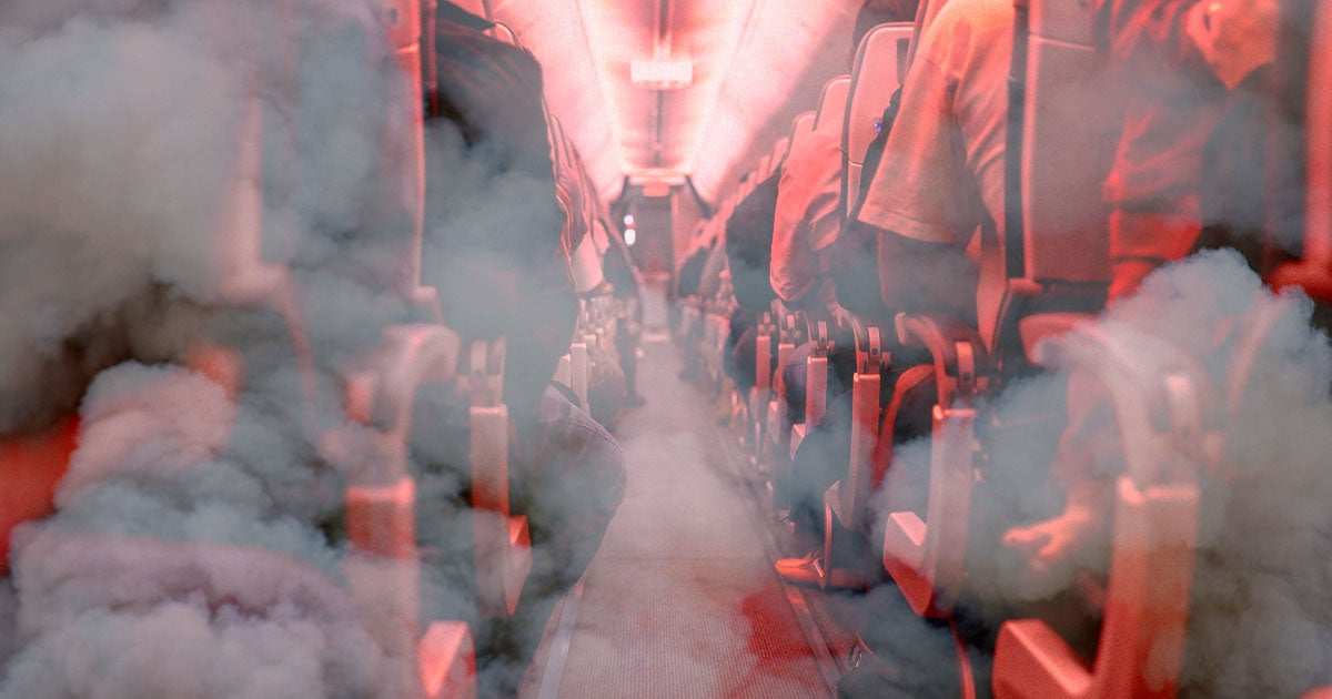
AI Generated Newscast About Airline Fumes: The Shocking Truth Airlines Don’t Want You to Know!
Ready for a jolt? An AI generated newscast about airline fumes has revealed a hidden danger lurking in the air aboard commercial flights—exposure to toxic fum ...
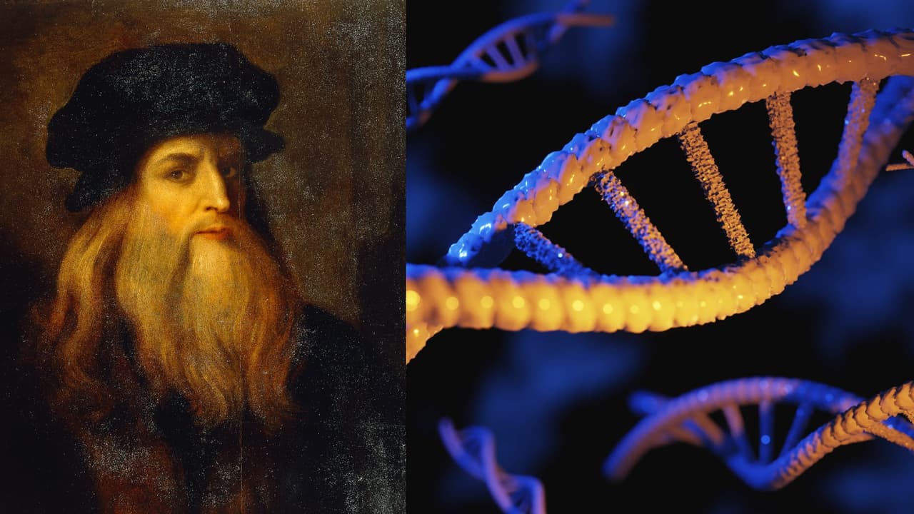
AI Generated Newscast About Da Vinci’s DNA: The Shocking Truth Scientists Just Uncovered!
What if AI generated newscast about Da Vinci’s DNA could finally unlock the secrets of genius? In a story straight out of a sci-fi movie, scientists are close ...
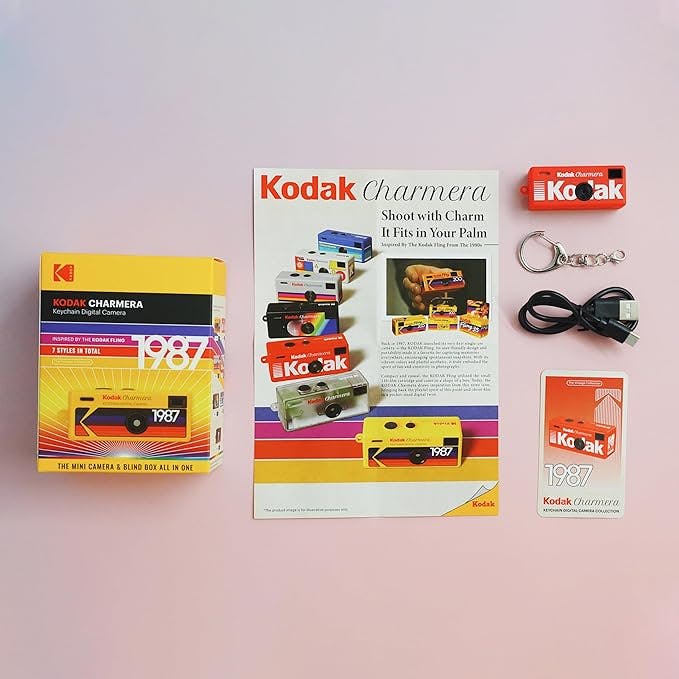
AI Generated Newscast About Kodak’s Shocking Comeback: Retro Camera Sells Out Instantly!
Would you ever believe Kodak could make a viral comeback in 2024? The AI generated newscast about Kodak reveals how the heritage film giant sold out its $29 ret ...
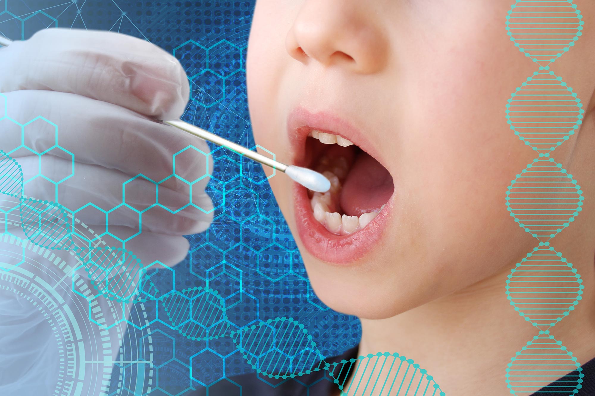
AI Generated Newscast About Inocles: Shocking DNA Discovery Changes Oral Health Forever!
Surprised by what's hiding in your saliva? Scientists have just discovered Inocles—giant, previously invisible DNA elements carried by about 74% of people—w ...

AI Generated Newscast About Anti-Ageing Breakthrough Shocks Skincare World!
Could a natural blueberry extract finally erase your wrinkles? That’s the question raised by a groundbreaking AI generated newscast about anti-ageing, which d ...
News by Category

AI Generated Newscast About Flying Car Crash: Xpeng's Futuristic Dream Goes Up in Smoke!
Flying cars are supposed to be the future—so what happens when they literally crash and burn?During a rehearsal for the Changchun air show, two Xpeng Aeroht e ...
AI Generated Newscast About Tesla’s FSD Shocker—$12k Gamble Leaves Owners Stunned!
Would you spend $12,000 for a self-driving future, only to realize you’re not even close? That’s the shock Tesla owners are facing today.Elon Musk has admit ...
AI Generated Newscast About Strip Club Tax Bribery: Executives Busted in $8M Scandal!
Imagine dodging $8 million in taxes with free trips and private dances – only to have an AI generated newscast about your strip club scandal go viral.RCI Hosp ...
AI Generated Newscast About Alien-Looking Sea Babies—What Are These Xenomorph Larvae Hiding?
HOOK: An alien-like sea creature has kept its adult form hidden for over a century, baffling scientists!The latest research reveals that mysterious baby facetot ...
AI Generated Newscast About Asteroid 2025 FA22: NASA Warns of Close Encounter!
Brace yourselves: a giant asteroid is hurtling past Earth soon—are we truly safe? The AI generated newscast about asteroid 2025 FA22 reveals that this 520-foo ...
AI generated newscast about Star Going Supernova! V Sagittae’s Imminent Explosion Will Dazzle Earth
Could a cosmic explosion light up our sky brighter than the moon? The answer is yes, and it might happen soon! Scientists have cracked the secret of V Sagittae, ...
AI Generated Newscast About Solo Female Travel in India: Shocking Truth Revealed!
Would you dare to visit a place everyone warns you about? Em did—and what she discovered in Mumbai is eye-opening.This AI generated newscast about solo female ...
AI Generated Newscast About Burner Phones: Shocking Truth Behind Your Privacy Risks!
What if your phone could be used to track your every move—without you even knowing? This AI generated newscast about burner phones reveals how authorities wor ...
AI Generated Newscast About Chrome vs. Edge: Microsoft’s Shocking Browser War Escalates!
Is your browser keeping you safe, or just selling you a story? Microsoft is once again pushing hard for users to pick Edge over Chrome, using bold new ads and i ...